EDA Exploratory Data Analysis
Exploratory Data Analysis (EDA) is used on the one hand to answer questions, test business assumptions, generate hypotheses for further analysis. On the other hand, you can also use it to prepare the data for modeling. The thing that these two probably have in common is a good knowledge of your data to either get the answers that you need or to develop an intuition for interpreting the results of future modeling.
There are a lot of ways to reach these goals: you can get a basic description of the data, visualize it, identify patterns in it, identify challenges of using the data, etc.
Data Exploration Tools
Pandas Profiling
Generates profile reports from a pandas DataFrame. The pandas df.describe() function is great but a little basic for serious exploratory data analysis. pandas_profiling extends the pandas DataFrame with df.profile_report() for quick data analysis.
For each column the following statistics - if relevant for the column type - are presented in an interactive HTML report:
- Type inference: detect the types of columns in a dataframe.
- Essentials: type, unique values, missing values
- Quantile statistics: like minimum value, Q1, median, Q3, maximum, range, interquartile range
- Descriptive statistics: like mean, mode, standard deviation, sum, median absolute deviation, coefficient of variation, kurtosis, skewness
- Most frequent values:
- Histograms:
- Correlations: highlighting of highly correlated variables, Spearman, Pearson and Kendall matrices
- Missing values: matrix, count, heatmap and dendrogram of missing values
- Duplicate rows: Lists the most occurring duplicate rows
- Text analysis: learn about categories (Uppercase, Space), scripts (Latin, Cyrillic) and blocks (ASCII) of text data
Basic Usage
import numpy as np
import pandas as pd
from pandas_profiling import ProfileReport

# build dataframe
df = pd.DataFrame(np.random.rand(100, 5), columns=["a", "b", "c", "d", "e"])

# generate a report
profile = ProfileReport(df, title="Pandas Profiling Report", explorative=True)

# Save report
profile.to_file("your_report.html")

# As a string
json_data = profile.to_json()

# As a file
profile.to_file("your_report.json")

Working with Larger datasets
Pandas Profiling by default comprehensively summarizes the input dataset in a way that gives the most insights for data analysis. For small datasets these computations can be performed in real-time. For larger datasets, we have to decide upfront which calculations to make. Whether a computation scales to big data not only depends on it’s complexity, but also on fast implementations that are available.
pandas-profiling includes a minimal configuration file, with more expensive computations turned off by default. This is a great starting point for larger datasets.
# minimal flag to True
# Sample 10.000 rows
sample = large_dataset.sample(10000)

profile = ProfileReport(sample, minimal=True)
profile.to_file("output.html")
Privacy Features
When dealing with sensitive data, such as private health records, sharing a report that includes a sample would violate patient’s privacy. The following shorthand groups together various options so that only aggregate information is provided in the report.
report = df.profile_report(sensitive=True)
SweetViz
Sweetviz is an open-source python auto-visualization library that generates a report, exploring the data with the help of high-density plots. It not only automates the EDA but is also used for comparing datasets and drawing inferences from it. A comparison of two datasets can be done by treating one as training and the other as testing.
The Sweetviz library generates a report having: - An overview of the dataset - Variable properties - Categorical associations - Numerical associations - Most frequent, smallest, largest values for numerical features
import sweetviz
import pandas as pd
train = pd.read_csv("train.csv")
test = pd.read_csv("test.csv")

my_report = sweetviz.compare([train, "Train"], [test, "Test"], "Survived")
show_html() command:
# Not providing a filename will default to SWEETVIZ_REPORT.html
my_report.show_html("Report.html")

Dtale
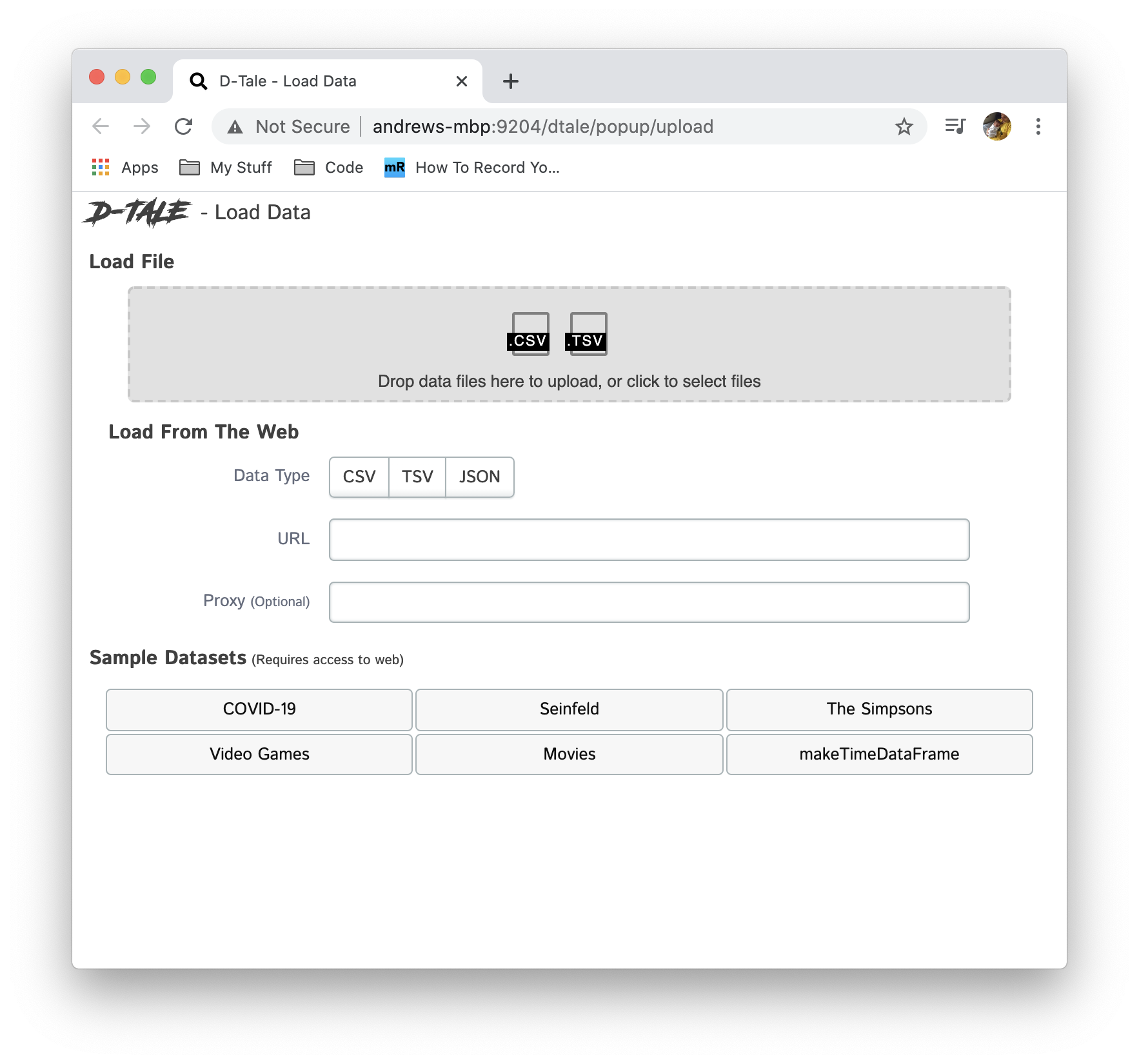
D-Tale is the combination of a Flask back-end and a React front-end to bring you an easy way to view & analyze Pandas data structures. It integrates seamlessly with ipython notebooks & python/ipython terminals. Currently this tool supports such Pandas objects as DataFrame, Series, MultiIndex, DatetimeIndex & RangeIndex.
To start without any data right away you can run dtale.show() and open the browser to input a CSV or TSV file.
import dtale
import pandas as pd

df = pd.DataFrame([dict(a=1,b=2,c=3)])
# Assigning a reference to a running D-Tale process
d = dtale.show(df)
Bulk
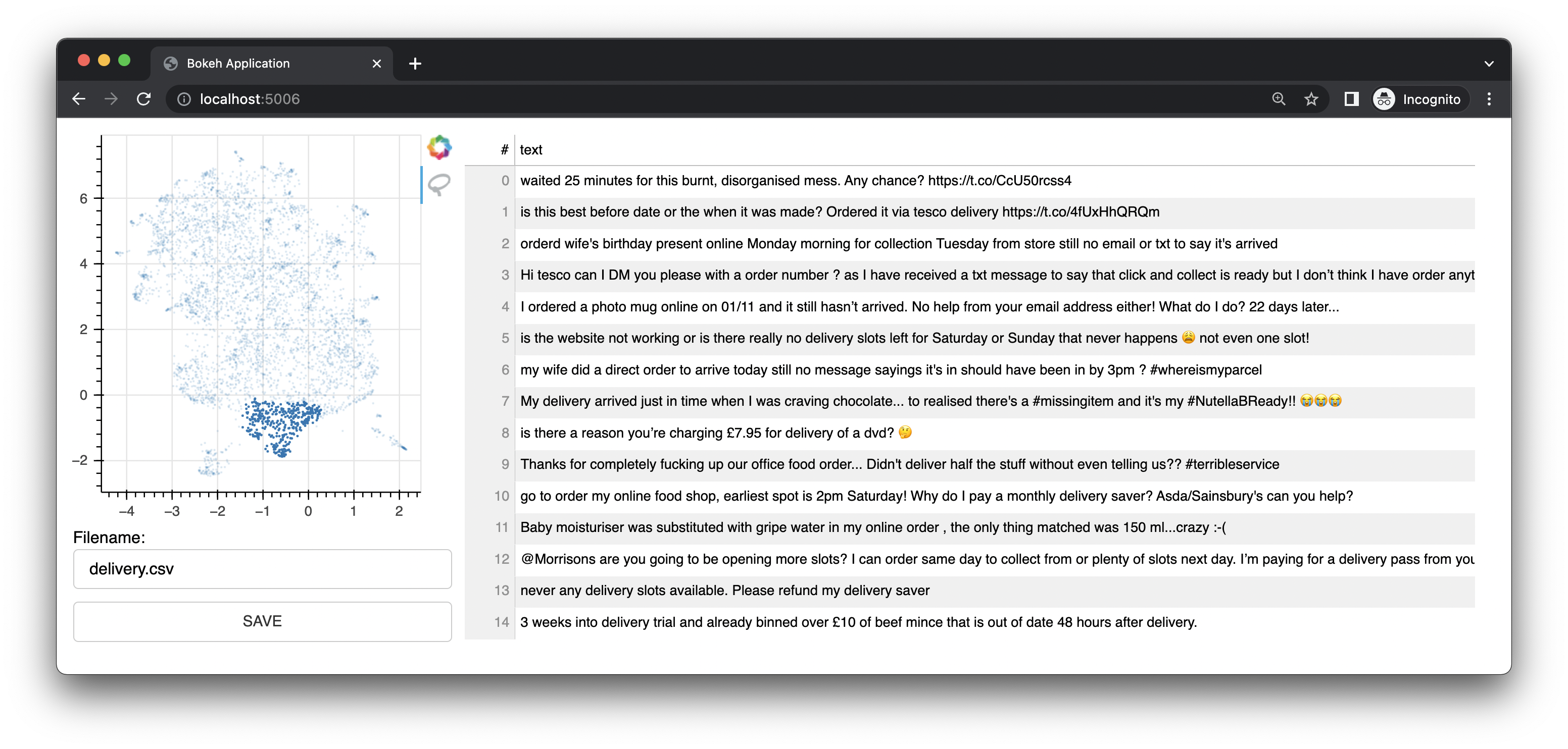
Bulk is a quick developer tool to apply some bulk labels. Given a prepared dataset with 2d embeddings it can generate an interface that allows you to quickly add some bulk, albeit less precice, annotations.
To use bulk for text, you'll first need to prepare a csv file first.
The example below uses embetter to generate the embeddings and umap to reduce the dimensions. But you're totally free to use what-ever text embedding tool that you like. You will need to install these tools seperately. Note that embetter uses sentence-transformers under the hood.
You can also use Bulk to explore semantic text data.
import pandas as pd
from umap import UMAP
from sklearn.pipeline import make_pipeline
from sklearn.linear_model import LogisticRegression


# pip install "embetter[text]"
from embetter.text import SentenceEncoder

# Build a sentence encoder pipeline with UMAP at the end.
text_emb_pipeline = make_pipeline(
  SentenceEncoder('all-MiniLM-L6-v2'),
  UMAP()
)

# Load sentences
sentences = list(pd.read_csv("original.csv")['sentences'])

# Calculate embeddings
X_tfm = text_emb_pipeline.fit_transform(sentences)

# Write to disk. Note! Text column must be named "text"
df = pd.DataFrame({"text": sentences})
df['x'] = X_tfm[:, 0]
df['y'] = X_tfm[:, 1]
df.to_csv("ready.csv")
python -m bulk text ready.csv
python -m bulk text ready.csv --keywords "foo,bar,other"
Data Exploration Manual
Python Pandas
import pandas as pd
df = pd.read_csv("path/to/file.csv")
df.describe()
More to come...
More to come...