Binning Data
When dealing with continuous numeric data, it is often helpful to bin the data into multiple buckets for further analysis. There are several different terms for binning including bucketing, discrete binning, discretization or quantization.
One of the most common instances of binning is done behind the scenes for you when creating a histogram. The histogram below of customer sales data, shows how a continuous set of sales numbers can be divided into discrete bins (for example: $60,000 - $70,000) and then used to group and count account instances.
Binning Data
Pandas cut
Pandas cut and qcut info is taken from pbpython
cut_labels_4 = ['silver', 'gold', 'platinum', 'diamond']
cut_bins = [0, 70000, 100000, 130000, 200000]
df['cut_ex1'] = pd.cut(df['ext price'], bins=cut_bins, labels=cut_labels_4)
| account number | name | ext price | cut_ex1 |
|---|---|---|---|
| 141962 | Herman LLC | 63626.03 | silver |
| 146832 | Kiehn-Spinka | 99608.77 | gold |
| 163416 | Purdy-Kunde | 77898.21 | gold |
| 218895 | Kulas Inc | 137351.96 | diamond |
| 239344 | Stokes LLC | 91535.92 | gold |
Pandas qcut
The pandas documentation describes qcut as a “Quantile-based discretization function.” This basically means that qcut tries to divide up the underlying data into equal sized bins. The function defines the bins using percentiles based on the distribution of the data, not the actual numeric edges of the bins.
The simplest use of qcut is to define the number of quantiles and let pandas figure out how to divide up the data. In the example below, we tell pandas to create 4 equal sized groupings of the data.
df['quantile_ex_1'] = pd.qcut(df['ext price'], q=4)
df['quantile_ex_2'] = pd.qcut(df['ext price'], q=10, precision=0)

df.head()
| account number | name | ext price | cut_ex1 | quantile_ex_2 |
|---|---|---|---|---|
| 141962 | Herman LLC | 63626.03 | (55733.049000000006, 89137.708] | (55732.0, 76471.0] |
| 146832 | Kiehn-Spinka | 99608.77 | (89137.708, 100271.535] | (95908.0, 100272.0] |
| 163416 | Purdy-Kunde | 77898.21 | (55733.049000000006, 89137.708] | (76471.0, 87168.0] |
| 218895 | Kulas Inc | 137351.96 | (110132.552, 184793.7] | (124778.0, 184794.0] |
| 239344 | Stokes LLC | 91535.92 | (89137.708, 100271.535] | (90686.0, 95908.0] |
Fisher-Jenks Algorithm
What we are trying to do is identify natural groupings of numbers that are “close” together while also maximizing the distance between the other groupings. Fisher developed a clustering algorithm that does this with 1 dimensional data (essentially a single list of numbers). In many ways it is similar to k-means clustering but is ultimately a simpler and faster algorithm because it only works on 1 dimensional data. Like k-means, you do need to specify the number of clusters. Therefore domain knowledge and understanding of the data are still essential to using this effectively.
The algorithm uses an iterative approach to find the best groupings of numbers based on how close they are together (based on variance from the group’s mean) while also trying to ensure the different groupings are as distinct as possible (by maximizing the group’s variance between groups).
import pandas as pd
import jenkspy
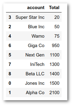
sales = {
'account': [
'Jones Inc', 'Alpha Co', 'Blue Inc', 'Super Star Inc', 'Wamo',
'Next Gen', 'Giga Co', 'IniTech', 'Beta LLC'
],
'Total': [1500, 2100, 50, 20, 75, 1100, 950, 1300, 1400]
}
df = pd.DataFrame(sales)
df.sort_values(by='Total')
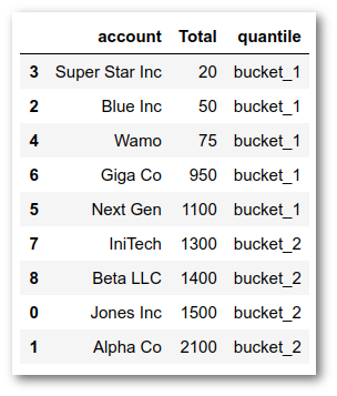
In order to illustrate how natural breaks are found, we can start by contrasting it with how quantiles are determined. For example, what happens if we try to use pd.qcut with 2 quantiles? Will that give us a similar result?
df['quantile'] = pd.qcut(df['Total'], q=2, labels=['bucket_1', 'bucket_2'])
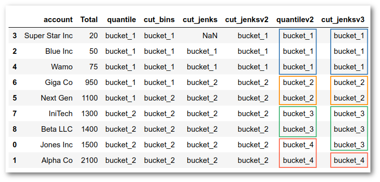
Just to get one more example, we can see what 4 buckets would look like with natural breaks and with a quantile cut approach:
df['quantilev2'] = pd.qcut(
    df['Total'], q=4, labels=['bucket_1', 'bucket_2', 'bucket_3', 'bucket_4'])

df['cut_jenksv3'] = pd.cut(
    df['Total'],
    bins=jenkspy.jenks_breaks(df['Total'], nb_class=4),
    labels=['bucket_1', 'bucket_2', 'bucket_3', 'bucket_4'],
    include_lowest=True)

df.sort_values(by='Total')